Test time training and RNN's
Background reading: Understanding RNN’s
Comparing RNN’s and attention.
RNN’s and attention are both sequence modelling techniques.
Where $N$ is length of the sequence, RNN’s exhibit $O(N)$ cost, and attention is $O(N^2)$ cost (as it multiplies $QK$ to lookup into $V$, where QKV are all projections of x).
Through a compression lens, RNN’s compress data differently to attention(?). Whereas attention can “shift back and forth”, RNN’s can only weight the outputs of the previous invocation.
an RNN layer’s ability to remember long context is limited by the amount of information its hidden state can store
Test-time training.
Test-time training (, video paper) is a new technique, which can be explained as:
- a formulation of an RNN where the hidden values (the recursions) $h$ are weights of a neural network $W$
- a new type of sequence modelling layer:
- a neural network inside a neural network
- the layer’s forward function performs training of the inner network, has its own learned learning rate and weight initialisation.
- the layer’s output is one inference of this inner network.
- the outer network’s training still takes the loss, which includes differentiating the forward function of the TTT layer, in itself, being a learning function. hence they refer to “gradients of gradients”.
With the definitions of an RNN:
- initial state:
s0 = vector() - update rule:
s_t = g((Whh * s_t-1) + (Whx * xt)) - output rule:
z_t = Why * s_t + Wyx
For a TTT layer:
- initial state:
W0 = f.params()- the initial state is the neural network’s weights
- update rule:
Wt = Wt−1 − η∇ℓ(Wt−1; xt)- update the current weight to the previous weights minus the learning rate times the gradient
- output rule:
zt = f(xt ; Wt)- output is one evaluation/inference of the network
The TTT layer is an RNN where the hidden units are weights of another neural network, and the output rule is an inference of that neural net.
The TTT layer performs the recurrence by running one training step on the weights.
The loss function so far is undefined - what is our learning objective for this TTT layer? It could be supervised, self-supervised, etc.
Basic objective function - reconstruction from noise.
In the TTT for video paper, they mention using an objective function that mirrors a reconstruction task like in denoising autoencoders:
$L(W;x_t) = || f(\hat{x_{t}}; W) - x_t || ^2 $
Translating this:
- process $x_t$ into corrupted input $\hat{x_{t}}$ (e.g. blur)
- loss = $|| f(\hat{x_{t}}; W) - x_t || ^2$
Objective function - low rank projection.
Maybe all information of $\hat{x_t}$ and the reconstruction label $x_t$ are necessary, so we can use a low rank projection instead. The low rank projections are referred to by their learned matrices $\theta_{Q},\theta_{K},\theta_{V}$ for the $x_t$, $\hat{x_{t}}$, and $z_t$ respectively.
As low rank projections change the dimension, the output rule is modified too:
$z_t = f(\theta{_Q}x_t ; W_t)$
There are a few more techniques they apply which are listed in the next section.
TTT-MLP.
The TTT they employ is a multi-layer perceptron.
Techniques.
Learnable $W_0$.
The TTT initialization $W_0$ is shared between all sequences. Empirically, we observe that learning $W_0$ significantly improves training stability
Learnable $\eta$
The learning rate is usually the most important hyper-parameter for gradient descent, so we experiment with learning the inner-loop learning rate $\eta$ in Equation 6 as part of the outer loop. We make $\eta$ a function of the input token (therefore different across time) for additional flexibility.
Concretely, we design η(x) = ηbase σ (θlr · x), where the learnable vector θlr is an outer-loop parameter, σ is the sigmoid function, and the scalar ηbase is the base learning rate, set to 1 for TTT-Linear and 0.1 for TTT-MLP.
Inner loop mini batch.
Given a TTT layer is a recurrent relation, where $h_i$ involves computing $h_{i-1}$, it cannot naively parallelized across tokens in a sequence.
They follow the standard mini batching you find in neural networks and apply it here.
-
Normal (fully sequential) update
- You have weights (W).
- For each new data point (x_t), you do
[ W \leftarrow W - \eta,\nabla\ell(W; x_t). ] - You can’t do two of these at once, because the second gradient needs the updated (W).
-
Write all updates at once
- If you start from (W_0) and do (T) steps, you get
[ W_T = W_0 - \eta\sum_{s=1}^T G_s,\quad G_s = \nabla\ell(W_{s-1}; x_s). ] - Now instead of “update–compute–update–compute…”, you can “compute all (G_s)” then subtract their sum.
- If you start from (W_0) and do (T) steps, you get
-
Mini-batch trick
- Pick a batch size (b) (e.g.\ 16).
- Split your (T) points into blocks of (b).
- For block 1 (steps 1…(b)): use (W_0) as the base. Compute in parallel
[ G_1 = \nabla\ell(W_0; x_1),;\dots,;G_b = \nabla\ell(W_0; x_b). ] - Then apply them in order by doing a cumulative sum:
[ W_1 = W_0 - \eta,G_1,; W_2 = W_1 - \eta,G_2,;\dots,; W_b = W_{b-1} - \eta,G_b. ] - For block 2 (steps (b+1)…(2b)): use (W_b) as base, compute those (b) gradients in parallel, then cumsum, and so on.
-
Why it helps
- You do (b) gradient computations at once instead of one by one.
- Larger (b): more parallel speed, but gradients get a bit “stale” (they all use the same base).
- Smaller (b): closer to true sequential updates but less speedup.
- They found (b=16) a good balance.
Gating.
Naively inserting TTT layers into a pre-trained network would dramatically worsen its predictions at the beginning of fine-tuning, when the TTT layers are randomly initialized. To avoid this degradation, we gate TTT with a learned vector $\alpha \in \mathbb{R_d}$ following standard practice:
$\texttt{gate}(TTT, X; α) = \texttt{tanh}(α) ⊗ \texttt{TTT}(X) + X$
We initialize all values in $α$ to 0.1, so the values in tanh($α$) are close to 0 (≈ 0.1) at the beginning of fine-tuning.
Bi-direction.
Diffusion models, including CogVideo-X, are non-causal, meaning that an output token zt can condition on all of x1, . . . , xT instead of only the past tokens x1, . . . , xt.
Standard trick - bi-direction.
$\texttt{TTT′}(X) = rev(\texttt{TTT}(rev(X)))$, where rev performs reverse.
Practice.
This is how they modify traditional transformer architectures.
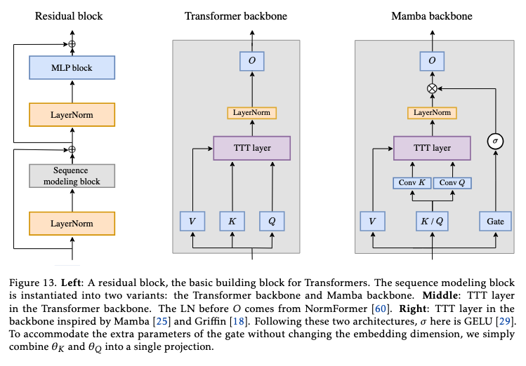
Translated to code:
# Normal backbone.
Xl = self_attn(LN(X))
Y = Xl + X # residual

# Modified backbone.
Xl = self_attn(LN(X))
Z = gate(TTT, Xl, a)
Zl = gate(TTT1, Z, b)
Y = Zl + X
–
Notes from the TTT paper.
- The difficulty with long context is inherent to the very nature of RNN layers: Unlike self-attention, RNN layers have to compress context into a hidden state of fixed size
- Tokens later in a sequence should be easier to predict on average, since they condition on more information. This is indeed the case for Transformer, whose average perplexity at each token index decreases throughout its 32k context. In contrast, the same metric plateaus for Mamba after 16k.
- On one hand, the main advantage of RNNs (vs. Transformers) is their linear (vs. quadratic) complexity. This asymptotic advantage is only realized in practice for long context, which according to Figure 12 is after 8k. On the other hand, once context is long enough, existing RNNs such as Mamba struggle to actually take advantage of the extra information being conditioned on